Any animal in a particular environment may be expected to grow at a certain rate, to live for a certain period, and to reproduce a certain number of offspring, usually spread over a certain span of its life. It is better to speak of the mean values for the population: there will be a mean rate of growth of individuals, a mean longevity which is more usefully considered as a distribution of ages at which different individuals die, and a mean fecundity which is more usefully considered as a mean birth rate at different ages of the mothers. The values of these means are determined in part by the environment and in part by a certain quality of the animal itself: its innate capacity for increase.
As I stated in the past, the growth of any population is a function of four demographic variables: births, deaths, ingress, and egress. For the sake of simplicity, let us ignore the last two, ingress and egress.
In an unlimited, constant, and favorable environment, the number of individuals of a species will increase exponentially. Under these theoretical conditions, virtually any species would cover the earth over a period of time. Of course, no animal or plant species has ever covered the earth (but it appears that we humans are trying). A point is reached when the population stops increasing, either because a greater density of individuals leads to greater mortality, or because of a decreased birth rate, or because conditions change and are no longer favorable.
The most common equations used in population ecology to simulate population growth stem in large part from a book by Lotka (1925), “Elements of Physical Biology.”
The equation for exponential rate of growth is:
Nt = N0ert , where t >= 0
where Nt is the number of individuals in the population at some time t, and N0 is the population density at some arbitrary set time, t = 0. The letter t represents units of time, usually years for deer and most often days for fruit flies. The units of t are set by the experimenter and convenience. In a deer population, t = 0 might be set at 1970. The year 1975 would then be equal to t = 5 if each unit of t equals one year. In other words, for the deer example, if we assumed or determined the herd was increasing exponentially, then starting from 1970, what would the herd size be in 1975?
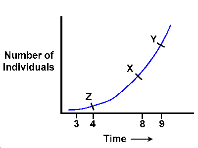
The above equation states that the size of the population at time t is equal to the population at the beginning (at t = 0) multiplied by e, the base of the natural logarithm (e = 2.7128. . .), raised to the rt power, where t is time and r is a constant that will be discussed later. There are two numbers free to vary: Nt and t. All other components always remain constant: e, r, and N0. In essence, the population is a function of how much time (t) has elapsed. The meaning of the constant r can be illustrated by the following figure:
At an arbitrarily chosen point X, a line is drawn contiguous to the point. The slope of the line is equal to the rate of change in the number of individuals in the population. The point X does not occupy any length of the curve or any period of time, so the rate is instantaneous at exactly X. Similar points can also be selected at Y and Z, and the contiguous lines drawn. At point Y, the increase in the number of individuals is greater than at point X, and in the same way the population at point X in time is increasing faster than at point Z. The number of individuals produced between t = 3 and t = 4 would be much fewer than those produced between t = 8 and t = 9. However, the ratio t=3/t=4 is equal to the ratio t=8/t=9, and this ratio will always remain the same for a single interval of time. The number of individuals added in one time interval rapidly increases with time, but the multiplication of the population in one time interval remains constant. The rate at which N, the number of individuals, changes as time changes can be represented as dN/dt, and for this curve:
dN/dt = rN
This can be recognized as a differential equation. At time t, the rate of increase in density is postulated to be equal to the constant r multiplied by the number of individuals present. When this equation is solved for explicit values of Nt, given an initial starting density N0, the following equation results:
Nt = N0ert
The constant r is a measure of the rate of multiplication of the population during an interval of time equal to 1. On the other hand, dN/dt represents the rate of change in number of individuals, and this rate constantly changes from instant to instant. The constant r is usually termed the intrinsic rate of increase. The value of r is a constant for a constant set of environmental conditions. If these conditions change, usually so will r.
Let us back up for a minute and define or derive some of the above to put it into a little more perspective.
Given:
N0 = population size at time 0
Nt = population size at time t
Bt = number of births in time interval t
Dt = number of deaths in time interval t
Ri = rate of population increase
R = finite rate (coefficient) of population growth
Then:
Rb = Bt / N0 = crude birth rate (Bt = RbN0)
Rd = Dt/N0 = crude death rate (Dt = RdN0)
Nt = N0 + (Bt - Dt)
= N0 + (RbN0 - RdN0)
= N0 (1 + Rb - Rd)
Ri = (Nt - N0) / N0
= [N0 (1 + Rb - Rd) - N0] / N0
Ri = Rb - Rd
The rate of population increase is equal to the crude birth rate minus the crude death rate. R = Nt / N0
= [N0 (1 + Rb - Rd)] / N0
= 1 + Rb - Rd
R = Ri + 1
The finite rate of growth, or the coefficient of growth, is equal to the rate of population increase plus 1.
It must be remembered that the rate of increase is defined only for a population with a stable age distribution, i.e., constant birth and death rates in age classes.
If we wish to describe the numerical increase in a population over a designated time period when crude birth and death rates are constant, we would use:
Nt = Rt N0
which is a description of geometric or exponential growth. A more frequent and mathematically more convenient notation to express the above function is the formula I gave you earlier:
Nt = N0ert
where er = R, or loge R=r
r = instantaneous rate of growth.
While r is the rate of increase of a population with a stable age distribution, R is the multiplication of the population in one interval of time. It is also a constant. If the population at time t consisted of 50 individuals, and at time t + 1 of 75 individuals, R = 1.5. In other words, the population has multiplied by a factor of 1.5 during the time t + 1. The intrinsic rate of increase in this example is loge 1.5 = 0.405.
It is perhaps easiest to conceive of r graphically under this exponential growth situation. Thus:
Nt = N0ert
ln (Nt) = ln (N0ert)
= ln (N0) + rt
= c + rt
This last equation is that of a straight line (y = a + bx) formed by plotting the logarithm of numbers in the population (ln Nt) against time (t); the slope of this line is r, the instantaneous rate of growth.
| There are three fairly common situations in nature where exponential growth may occur over appreciable periods of time: |
Where a species has been introduced by man into (or has naturally colonized) a new and acceptable geographic area.
Where a species has been greatly depressed by man’s activities and such activities cease.
Where a species naturally undergoes marked fluctuations and population growth consequently begins from densities that are very low relative to environmental carrying capacity.

Updated 06 August 1996