WLF 448: Fish & Wildlife Population Ecology
Lecture Notes IX, Fall 1996
POPULATION GROWTH IN LIMITED ENVIRONMENTS
by S. R. Peterson (1977)
Introduction
Up until now, in this section of population growth, I have
discussed growth in an unlimited environment. This phenomenon
is essentially described using an exponential function. In
the equation Nt = N0ert the
calculation of r assumes the environment is not limiting. But
what if some part of the environment is limiting? As we know,
populations in actuality do not increase forever, because
something or a combination of things (limiting factors) hold
down population growth.
Birch’s Study (1953)
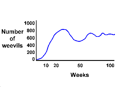
Birch did a very interesting experiment with weevils (Calandra
oryzae). He introduced a female and a male weevil into 12
grams of wheat at a constant temperature and humidity, and
followed the change in number of adults for 100 weeks (almost
2 years). There were, of course, fluctuations in the food
supply as it was eaten, but the food supply was more or less
constant.

Features of the experiment:
-
At the beginning, the growth of the
population is almost exponential, increasing close to
the intrinsic rate of increase.
-
After the tenth week, the rate of
increase begins to slow, and at about the twentieth
week the population plateaus.
-
After that, the population
fluctuates around a mean of about 700.
Other experiments of this nature have shown similar
results.
I previously pointed out that the intrinsic rate of
increase is equal to r, which equals the intrinsic birth rate
(b) minus the intrinsic death rate (d). In an unlimited,
constant environment, the birth rate and death rate do not
change, and consequently neither does r. But observations
such as Birch’s experiment indicate that the rate of
population growth progressively slows as the number of
individuals reaches maximum possible density. Somehow, the
increase in density causes the birth rate to decrease, the
death rate to increase, or both. At the plateau, b equals d
and therefore r equals 0.
Logistic Equation
The initial growth of a population up to the plateau is
roughly an S-shaped curve. The earliest attempt to simulate
this curve was the logistic equation of Verhulst (1839). The
S-shaped or logistic curve differs from the geometric curve
in two ways:
-
It has an upper asymptote (the curve
does not exceed a certain maximum level), and
-
it approaches this asymptote
smoothly, but abruptly. In fact, when you divide the
curve at its inflection point, the upper and lower
halves are mirror images of each other.
The reasoning behind the logistic curve is simple. The
population density increases but at higher densities, the rate
of increase decreases. At some maximum density, it
does not increase at all.
The logistic growth equation has proven remarkably useful
in population ecology. The equation seems to describe growth
reasonably well for a number of populations. Yeast and
protozoan growth curves, for example, fit the model quite
well, as to a less precise degree do those of same metazoans.
Gause found reasonable fits for Paramecium and for
flour beetles (Tribolium), and Pearl found the
logistic equation to fit quite accurately the growth in Drosophila
melanogaster populations.
While growth curves similar to those predicted by the
logistic growth model are occasionally found, most metazoans
do not show very good fits to the equation. In fact, growing
metazoan populations usually show quite regular damped
oscillations. These oscillations appeared under quite
constant laboratory conditions, and therefore were not due to
environmentally induced fluctuations in r. The question is,
why should the oscillations occur?
As Krebs point out, the simplest way to produce an
S-shaped curve is to introduce into our geometric equation
(the integral of dN/dt, Nt = N0ert)
a term that will reduce the rate of increase as the
population builds. We also want to reduce the rate of
increase in a smooth manner, and this is accomplished by
making each individual added to the population reduce the
rate of increase an equal amount. The classic way of
describing the progressively increasing environmental
resistance to further growth is shown by the addition of the
“dampening factor” (X - N) / K to the above
differential equation.
Thus, dN/dt = rN [(K-N)/K]
r = growth rate constant
K = the maximum number of individuals that the
given environment can support, i.e. the upper limit
of population growth
Basically, this equation states that:
Rate of increase of population per unit of time
(dN/dt) = Innate capacity for increase (rmax)
x Population size (N) x Unutilized opportunity for growth
(K-N / K).
Integration gives an algebraic form of the
so-called logistic equation:
Nt = K / (1 + A e-rt), where A =
constant
This equation can be written another way by rearranging
the terms:
ln [(K-N) / N] = a - rt
This is also the equation of a straight line in which the
coordinates are:
Y coordinate = ln (K-N / N)
X coordinate = time
Two attributes of the logistic curve make it
attractive:
-
mathematical simplicity, and
- apparent reality.
The biological meaning of K is
essentially the density at which the space being studied
becomes “saturated” with organisms (the carrying
capacity).
Assumptions of the logistic equation (Krebs):
-
The population has an initially stable
age distribution
-
The density has been measured in
appropriate units.
-
There is a real attribute of the
population corresponding to r, the intrinsic rate of
increase.
-
*The relationship between density and
the rate of increase is linear – probably violated
in many growing populations.
-
* The depressive influence of density on
the rate of increase operates instantaneously, without
any time lapse. Highly unlikely that in organisms with
complex life cycles the rate of population increase could
respond instantaneously.
At one time, it was suggested that the logistic curve per
se described a fundamental law of population growth. This
viewpoint has largely been abandoned over the years as early
predictions about human population growth (rates and upper
limits) proved grossly incorrect and more field data on
growth in other species became available.
Value of the logistic theory
 |
The real value of logistic theory is
that it introduces us to such concepts as density-dependence
and mean population level. |
 Return to Lecture Notes IX: Population
Growth - Limited Environments.


Updated 06 August 1996


