EnvS 541

ENVS 541
Sampling and Analysis of Environmental Contaminants

ANOVA Post Hoc Tests

This is some example output from Systat showing how to carry out tests after an ANOVA to see which of the factor level means is different from each other.  Remember, doing all pairwise comparisons using simple t tests corrupts the significance levels.

Here’s what the Systat manual has to say:

The results in an ANOVA table serve only to indicate whether means differ significantly or not.  They do not indicate which means differ from another.  To report which pairs of means differ significantly, you might think of computing a two-sample t test for each pair; however, do not do this.  The probability associated with the two-sample t test assumes that only one test is performed.  When several means are tested pairwise, the probability of finding one significant difference by chance alone increases rapidly with the number of pairs.  If you use a 0.05 significance level to test that means A and B are equal and to test that means C and D are equal, the overall acceptance region is now 0.95*0.95 or 0.9025.  Thus, the acceptance region for two independent comparisons carried out simultaneously is about 90%, and the critical region is 10% (instead of the desired 5%).  For six pairs of means tested at the 0.05 significance level, the probability of a difference falling in the critical region is not 0.05 but 1-(0.95)6 = 0.265.  For 10 pairs, this probability increases to 0.40.  The result of following such a strategy is to declare differences as significant when they are not.

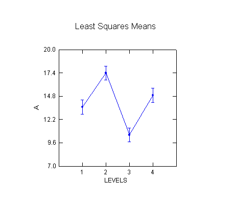
Here’s some data from 4 levels of a factor with 10 data points per level:

10            1
14            1  
15            1  
13            1  
17            1  
12            1  
19            1  
15            1  
10            1  
11            1  
15            2  
18            2  
17            2  
16            2  
18            2  
16            2  
19            2  
22            2  
19            2  
14            2  
10            3  
08            3  
12            3  
11            3  
14            3  
13            3  
07            3  
10            3  
11            3  
09            3  
13            4  
15            4  
14            4  
17            4  
16            4  
13            4  
15            4  
19            4  
11            4
16            4  
 

Here’s the output from Systat for the ANOVA:

Effects coding used for categorical variables in model.

Categorical values encountered during processing are:  
LEVELS (4 levels)

 This shows the means and their standard errors:

Durbin-Watson D Statistic     2.047  
First Order Autocorrelation   -0.056  
COL/  
ROW LEVELS 
  1  1 
  2  2 
  3  3 
  4  4  
Using least squares means.
 

Bonferroni Adjustment.  
Matrix of pairwise comparison probabilities:

So, the mean of level 1 is significantly different from level 2, barely different from level 3, not different from level 4. Level 2 is different from level 3 but not from level 4.  Level 3 is different from level 4.