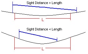
 Sag vertical curves are curves that connect descending grades, forming a bowl or a sag. Designing them is is very similar to the design of crest vertical curves. Once again, the sight distance is the parameter that is normally employed to find the length of the curve. When designing a sag vertical curve, however, the engineer must pay special attention to the comfort of the drivers. Sag vertical curves are characterized by a positive change in grade, which means that vehicles traveling over sag vertical curves are accelerated upward. Because of the inertia of the driver's body, this upward acceleration feels like a downward thrust. When this perceived thrust and gravity combine, drivers can experience discomfort. The length of sag vertical curves, which is the only parameter that we need for design, is determined by considering drainage, driver comfort, aesthetics, and sight distance. Once again, the aesthetics and driver comfort concerns are normally automatically resolved when the curve is designed with adequate sight distance in mind. Driver comfort, for example, requires a curve length that is approximately 50% of the curve length required for the sight distance. Drainage may be a problem if the curve is quite long and flat, or if the sag is within a cut. For more information on these secondary concerns, see your local design manuals. The theory behind the sight distance calculations for sag vertical curves is only slightly different from that for crest vertical curves. Sag vertical curves normally present drivers with a commanding view of the roadway during the daylight hours, but unfortunately, they truncate the forward spread of the driver's headlights at night. Because the sight distance is restricted after dark, the headlight beams are the focus of the sight distance calculations. For sight distance calculations, a 1° upward divergence of the beam is normally assumed. In addition, the headlights of the vehicle are assumed to reside 2 ft above the roadway surface. As with crest vertical curves, these assumptions lead to two possible configurations, one in which the sight distance is greater than the curve length, and one in which the opposite is true. The figure below illustrates these possibilities.
If S > L then
If S < L then
L = Curve length (ft) S = Sight distance (ft) (normally the stopping sight distance) B = Beam upward divergence (°) (normally assumed as 1°) H = Height of the headlights (ft) (normally assumed as 2 ft) A = Change in grade (|G2-G1| as a percent) The stopping sight distance is normally the controlling sight distance for sag vertical curves. At decision points, the roadway should be illuminated by other means so that the sight distance of the driver is extended. Where possible, increased curve length may also be provided. Highway overpasses or other obstacles can occasionally reduce the sight distance on sag vertical curves. In these instances, separate equations should be used to determine the correct curve length. These equations are readily available in design manuals. At this point, you have all of the information that you need to develop the precise layout of your vertical curve. The parabolic curve calculations are identical for sag and crest vertical curves. Just remember to use the appropriate positive or negative values for the participating grades.
|