Gravity Model

A study area consists of three zones. The data have been determined as shown in the following tables. Assume a K_ij =1.

Zone Productions and Attractions

Travel Time between zones (min)

Travel Time versus Friction Factor

Determine the number of trips between each zone using the gravity model formula and the data given above. Note that while the Friction Factors are given in this problem, they will normally need to be derived by the calibration process described in the Theory and Concepts section.

[Solution Shown Below]

Solution

First, determine the friction factor for each origin-destination pair by using the travel times and friction factors given in the problem statement.

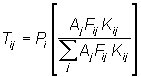
Once you have the friction factors for each potential trip, you can begin solving the gravity model equation as shown below. Solving for the A*F*K term in a tabular form makes this process easier. Study the equation below and the following table.

Where:
T_ij = number of trips that are produced in zone I and attracted to zone j
P_i = total number of trips produced in zone I
A_j = number of trips attracted to zone j
F_ij = a value which is an inverse function of travel time
K_ij = socio economic adjustment factor for interchange ij

Once the A*F*K terms for each origin-destination are tabulated, you can insert these values into the gravity model equation and determine the number of trips for each origin-destination. The following table illustrates this.

Zone to Zone First Iteration:

Since the total trip attractions for each zone don’t match the attractions that were given in the problem statement, we need to adjust the attraction factors. Calculate the adjusted attraction factors according to the following formula:

A_jk =

Where:
A_jk = adjusted attraction factor for attraction zone (column) j iteration k.
A_jk = A_j when k=1
C_jk = actual attraction (column) total for zone j, iteration k
A_j= desired attraction total to attraction zone (column) j
j= attraction zone number
n= number of zones
k = iteration number

To produce a mathematically correct result, repeat the trip distribution computation using the modified attraction values.

For example, for zone 1:

 Zone to Zone Second Iteration:

Upon finishing the second iteration, the calculated attractions are within 5% of the given attractions. This is an acceptable result and the final summary of the trip distribution is shown below.

The resulting trip table is: