Measuring Frequency

Basics of Frequency Analysis

Frequency assessment of plant communities is most often used to compare:

• Changes in a site over years, or
• Differences between sites

I most cases we want to know if the times or sites are “significantly different.” This comparison of frequency data is most often conducted with a Chi Square Analysis.

Detail Description of Chi Square Analysis

The Measuring and Monitoring book that we are using for this class has a complete and detailed description of how a chi-square test can be used to test differences for two populations.

• Pages in Measuring and Monitoring relevant to Chi Square test.

Data Analysis with Chi Square

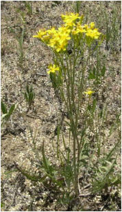
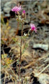
For example: Assume we examined 150 plots on bunchgrass sites with south-facing slopes in Idaho and Oregon. On these sites we calculated a frequency of 36% (present 54 out of 150 plots) for Indian Paintbrush (Castilleja linariifolia) using a 1 m² plot. Then, we also examined 150 plots on sites with north-facing aspects and we found that the frequency of paintbursh was 48% (72 plots out of 150). What we really want to know is – does a difference of 12% indicate a real, or significant, difference in the amount of paintbrush frequency and abundance on north and south facing slopes. A Chi Square can give us a way to judge if the sites are really “different.”

• Data are arranged in rows of what was observed and columns of the treatment we want to examing.  In this case our "treatment" is south- versus north-faxing slope.

• Data from field = "Observed" either present or absent in the plots examined.

• The number "Expected" is based on an equation to estimate the amount you would expect if there was no treatment effect.
  Expected= Total occurrences Observed for both treatments × total plots in on treatment ÷ Total plots examine in both sites.
  Easily calculated in a table as Expected Value = (Row Total × Column Total) ÷ Grand Total

Chi Square Formula:

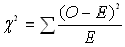Where: χ2 = the chi square statistic (calculated value) ∑ = sum of the variables O = Observed Value E = Expected Value

In Example Above:

A calculated χ2 statistic of 4.4 can then be compared to a critical or table χ2 statistic to determine of the values in the comparison are different. In other words, is the χ2 statistic that we generated large enough to be "significant."

Evaluating a χ2 Statistic:

Look in a Chi Square Table to determine the appropriate χ2 critical value.  To find a value in a chi-square table you much determine the v (or degrees of freedom; df) for your comparison:

v = (r-1)(c-1) or v = (number of rows in comparison - 1) (number of columns - 1)
In our example, for a 2 x 2 comparison, v = (2-1)(2-1) = 1

• If we use a P-threshold (or α) of 0.10, the χ2 critical or table value is 2.706.
• The χ2 statistic calculated for these data was 4.4.
• The null hypothesis is that there is no difference between or among samples in the comparison. (In other words, the null hypothesis in this example. is that there is no difference in the frequency of paintbrush on north- and south-facing slopes).
• If the value calculated is greater than the table value, we reject the null hypothesis
• In this example,  4.4 is > 2.7 so we reject the null hypothesis, and conclude that the frequency of paintbrush is different between north- and south-facing slopes.

**Note on Chi-Square Tables - 
1) Follow this link to a common Chi-Square Table
2) You can also enter you calculate chi-square value in a Chi-Square Calculator
3) Excel also has a function to calculate chi-square (check the help button in excel)

Summary Questions

1. What is the null hypothesis for a Chi Square test?
2. What relationship between between a calculate χ2 and a critical (or table) χ2 will cause one to reject the null hypothesis?

Advanced Question

1. In the attached example, calculate the frequency for 4 plot sizes for the following species in the data:

   Bluebunch Wheatgrass	Tappertip Hawksbeard	Spotted Knapweed	Lost River Silene

2. Determine the appropriate frame size to compare each of these species from 1995 to 2003.
   Click here for answer
3. Use a Chi-Square analysis of each species for the appropriate frame size to determine if the frequency of the plant has changed between 1995 and 2003.  Look on separate tabs in spreadsheet with answer for question 2, to see chi-square tests for each species.