| Lecture | Date | Topic(s) | Data/Assignment | Reading | Computer Program |
|---|---|---|---|---|---|
| 1a,b,c | 1/10 | Introduction; Review of simple and multiple regression; Matrix and R, SAS/IML review; Review of statistical inference for regression |
Short
answers due lecture 2 Hw1, due lecture 4 Some Hw1 hints |
Chapters 5-6 | Davis.txt prestige.txt Davis SAS program Davis SAS output R Davis code Prestige SAS program Prestige SAS output R Prestige code IML intro IML SAS output R Matrix code |
| 2 | 1/15 | Review of statistical inference for
regression; ANCOVA, the principle of marginality |
Chapters 6-7 | Drop
test SAS Program Ancova SAS program Ancova SAS output SAS-text comparison R Ancova code |
|
| 3a,b | 1/17 | ANCOVA, the principle of marginality; Analysis of variance |
Chapter 7-8 | Moore.txt Anova SAS program Anova SAS output R Anova code |
|
| 4a,b,c | 1/22 | ANOVA; Statistical theory for linear models | Hw1 due | Chap. 9.1-9.2 | |
| 5a,b,c | 1/24 | Statistical theory for linear models | Hw2, due lecture 8 | Chap. 9.1-9.2 | |
| 6a,b | 1/29 | Homework 1 review; More statistical theory for linear models; Properties of the least-squares estimator |
Chap. 9.3-9.4 | ||
| 7 | 1/31 | Properties of the least-squares estimator; Inference for several coefficients |
Some Hw2 hints | Chap. 9.3-9.4 | Gen Lin Hyp SAS
code; GLH SAS output R GLH code |
| 8a, b | 2/5 | Inference for coefficients; Joint Confidence Regions; Random regressors; Specification error; Confidence and prediction intervals |
Hw2 due |
Chap. 9.4 -9.8 | Joint Conf.
Ellipse 1; Joint Conf. Ellipse 2; Crime data info; Crime data; R Conf. Ellipse code |
| 9a,b | 2/7 | Vector Geometry of Linear Models | Exam
1 take home; Anova data |
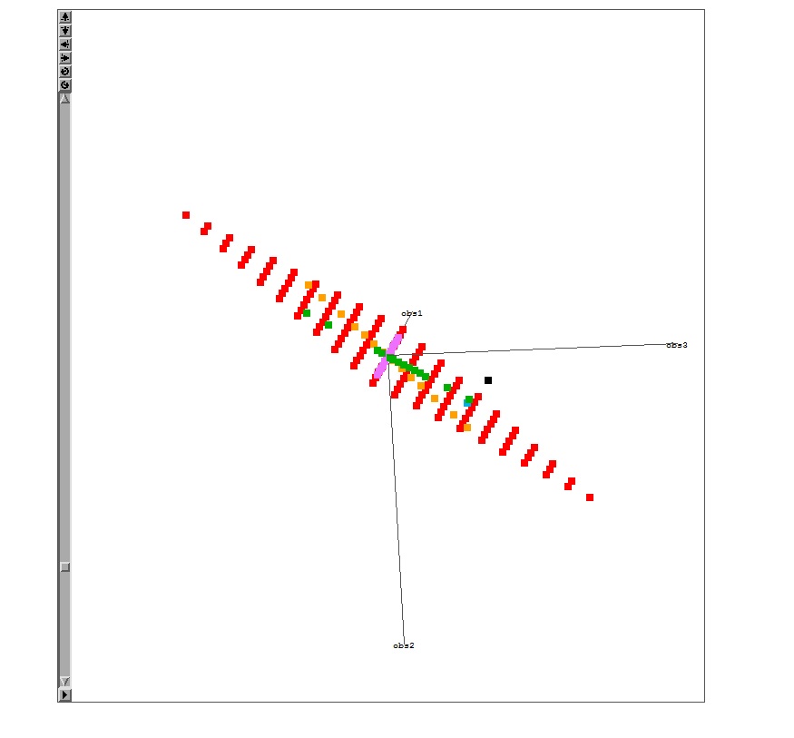
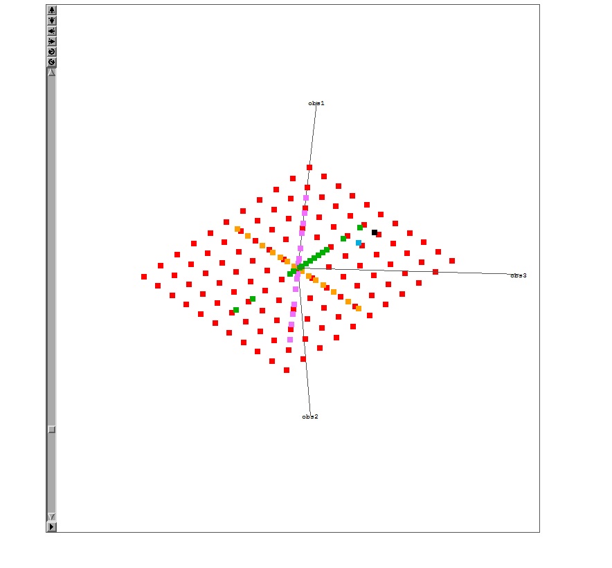
Chap. 10.1-10.4 | Geometry
R code Geometry SAS code; Geom. SAS Fig1 ; Geom. SAS Fig2 ; LS Geometry figure |
| 10 | 2/12 | Homework 2 review; Vector Geometry of Linear Models |
Chap. 10.1-10.4 | Figure 10.7
R code Anova R code Anova Geometry SAS code ; Anova SAS 1; Anova SAS 2 |
|
| 11a,b,c | 2/14 | Vector Geometry of Linear Models; Statistical theory for linear models; Theory about TSS decomposition |
Chap. 10 and extra |
Quadratic form SAS code | |
| 2/19 | Exam 1 | ||||
| 12a,b | 2/21 |
Hat values and residuals; Measuring Influence |
Hw3, due lecture 16 | Chap. 11-1-11.5 | Duncan.txt;
Hat, resid SAS program; Hat, resid SAS output; R Hat, resid code |
| EA1, 13 | 2/26 | Exam 1 Review; Joint Influence | Chap. 11.6-11.8 | Partial Reg.
SAS code; Partial Reg. SAS output; R Partial Reg. code; R Forward Search code; R Forward Search Figure |
|
| 14a, b | 2/28 | The normality assumption; The constant variance assumption |
Chap. 12.1-12.2 | SLID1.txt; Quantile/KDE SAS program; Quantile/KDE SAS output; R quantile/KDE code; WLS SAS code; WLS SAS output; R WLS code; Sandwich SAS code; Sandwich SAS output; R Sandwich code |
|
| 15a,b,c,d | 3/5 | The linearity assumption; Discrete data; Box-Cox transformations |
Chap. 12.2-12.6 | Part. resid.
example SAS; Part. resid SAS output; SLID part.res. SAS code; SLID part. res. output; R part. res. code; Vocabulary.txt; discrete data SAS code; discrete data SAS output; R discrete data code; Box-Cox SAS code; Box-Cox output; R Box-Cox code |
|
| 16a,b,c, | 3/7 | Box-Tidwell transformations; More tests for constant variance; Structural Dimension |
Hw3 due ; Hw4, due lecture 21 | Chap. 12.5-12.6 | Box-Tidwell
SAS code; Box-Tidwell output; R Box-Tidwell code; BFox.txt |
| 3/11-3/15 | Spring break - no classes | ||||
| 17a,b,c,d | 3/19 | Hw3 review; Detecting Collinearity; Model Respecification; Variable Selection; |
Chap. 13.1-2 | Collinearity SAS
code; Collinearity output; R Collinearity code Model selection SAS code; Model selection output; R Model selection code; |
|
| 18a,b | 3/21 | Variable Selection Methods | Chap. 13.1-2 | Ridge regr. SAS code;
Ridge regression output; R Ridge reg. code; ESL example SAS code; ESL data |
|
| 19 | 3/26 | Nonlinear Regression | Chap. 17.4 | Nonlinear regr. SAS
code; Nonlinear regr. output; R Nonlinear code |
|
| 20 | 3/28 | Models for Dichotomous Data | Hw4 due; Exam 2 take home |
Chap. 14.1 | Cereals.txt; Simple Logistic Reg.code; SAS Logistic Reg output; R Logistic Reg. code |
| 21 a,b | 4/2 | Models for Dichotomous Data; Generalized Linear Models |
Chap. 14.1, 15.1 |
SLID-women.txt;
Logistic Reg. SAS code; Logistic Reg. SAS output; R Logistic Reg. code |
|
| 22 | 4/4 | Homework 4 Review; The Structure of Generalized Linear Models |
Chap. 15.1-2 | SAS
Deviance calculation; SAS Dev. Calc. output; R code |
|
| 4/9 | Exam 2 | ||||
| 23a,,b,c,d | 4/11 | The Structure of Generalized Linear Models;
GLMs for Count Data |
Chap. 15.1-2 | Ornstein.txt; Poisson Reg. SAS code; Poisson Reg. output ; R Poisson Reg. code ; IWLS SAS code; IWLS SAS output |
|
| EA2, 24 a,b,c |
4/16 | Exam 2 Review; Statistical Theory for Generalized Linear Models |
Hw5, for review | Chap. 15.3 | Delta method SAS
code; Delta method R code |
| 25 | 4/18 | Diagnostics for Generalized Linear Models | Chap. 15.3-4 | Deviance
calculation SAS code; Deviance output; GLM Diag. SAS code; GLM Diag. output; R GLM Diag. code |
|
| 26 | 4/23 | Introduction to Mixed Models | Mixed SAS code; Mixed SAS output; R Mixed code |
||
| 27 | 4/25 | Mixed Models | Exam 3 take home;
baseball data; prob 4 data |
Chap. 23.1-6 | SAS
School code; SAS Eating code; R Eating code |
| 28 | 4/30 | Student talks | |||
| 29 | 5/2 | Homework 5 review | |||
| Finals week |
Office hours: TBD |
. | . | ||
| Finals week |
Final Exam |
. | . | ||